Digit recognition with SQFA

In this tutorial, we compare SQFA to standard dimensionality reduction methods using the digit recognition dataset Street View House Numbers (SVHN). We compare SQFA to different standard methods available in the sklearn library: PCA, LDA, ICA and Factor Analysis. To compare the methods, we test the performance of a Quadratic Discriminant Analysis (QDA) classifier trained on the features learned by each method.

We will show that SQFA features outperform those learned by the other methods, while being learned in approximately the same time as LDA filters.

Street View House Numbers (SVHN) dataset

The SVHN dataset consists of images of house numbers taken from Google Street View, and while it has a similar structure to the MNIST dataset, it is significantly harder. Let’s load the dataset and visualize some of the images.

import torch
import matplotlib.pyplot as plt
import torchvision

torch.manual_seed(2)

# Download and load training and test datasets
trainset = torchvision.datasets.SVHN(root='./data', split='train', download=True)
testset = torchvision.datasets.SVHN(root='./data', split='test', download=True)

# Convert to PyTorch tensors, average channels and reshape
n_samples, n_channels, n_row, n_col = trainset.data.shape
x_train = torch.as_tensor(trainset.data).float()
x_train = x_train.mean(dim=1).reshape(-1, n_row * n_col)
y_train = torch.as_tensor(trainset.labels, dtype=torch.long)
x_test = torch.as_tensor(testset.data).float()
x_test = x_test.mean(dim=1).reshape(-1, n_row * n_col)
y_test = torch.as_tensor(testset.labels, dtype=torch.long)

# Scale data and subtract global mean
def scale_and_center(x_train, x_test):
    std = x_train.std()
    x_train = x_train / (std * n_row)
    x_test = x_test / (std * n_row)
    global_mean = x_train.mean(axis=0, keepdims=True)
    x_train = x_train - global_mean
    x_test = x_test - global_mean
    return x_train, x_test

x_train, x_test = scale_and_center(x_train, x_test)

# See how many dimensions, samples and classes we have
print(f"Number of dimensions: {x_train.shape[1]}")
print(f"Number of samples: {x_train.shape[0]}")
print(f"Number of classes: {len(torch.unique(y_train))}")
print(f"Number of test samples: {x_test.shape[0]}")

# Visualize some of the centered images
names = y_train.unique().tolist()
n_classes = len(y_train.unique())
fig, ax = plt.subplots(2, n_classes // 2, figsize=(8, 4))
for i in range(n_classes):
    row = i // 5
    col = i % 5
    ax[row, col].imshow(x_train[y_train == i][20].reshape(n_row, n_col), cmap='gray')
    ax[row, col].axis('off')
    ax[row, col].set_title(names[i], fontsize=10)
plt.tight_layout()
plt.show()

Number of dimensions: 1024
Number of samples: 73257
Number of classes: 10
Number of test samples: 26032

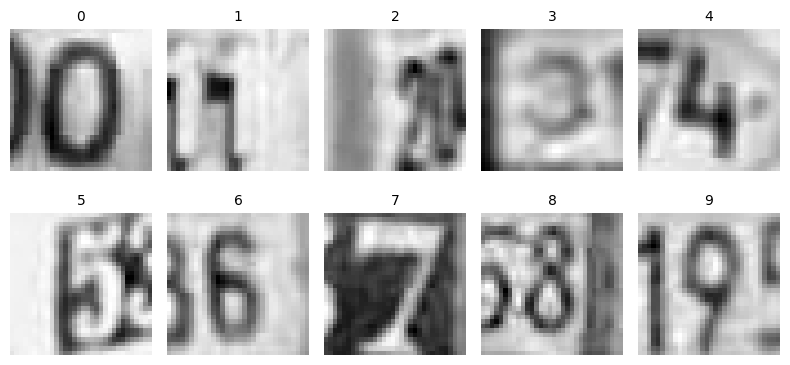
We see that we have 10 classes and that the training data consists of 73257 samples of 1024 dimensions. We will now learn 9 filters for this dataset using each of the different dimensionality reduction methods.

Maximum number of filters

A limitation of LDA is that it can learn a maximum of \(c-1\) filters, where \(c\) is the number of classes. This is the reason why we learn 9 filters in this tutorial. SQFA does not have this limitation.

from sklearn.discriminant_analysis import LinearDiscriminantAnalysis, QuadraticDiscriminantAnalysis
from sklearn.decomposition import PCA, FastICA, FactorAnalysis
from sklearn.cross_decomposition import CCA
import sqfa
import time

N_FILTERS = 9

# TRAIN THE DIFFERENT MODELS

# Train PCA
pca = PCA(n_components=N_FILTERS, svd_solver='covariance_eigh') # Fastest solver
start = time.time()
pca.fit(x_train)
pca_time = time.time() - start
pca_filters = pca.components_

# Train LDA
shrinkage = 0.8  # Set to optimize LDA performance and have smoother filters
lda = LinearDiscriminantAnalysis(solver='eigen', shrinkage=shrinkage)
start = time.time()
lda.fit(x_train, y_train)
lda_time = time.time() - start
lda_filters = lda.coef_[:N_FILTERS]

# Train ICA
ica = FastICA(n_components=N_FILTERS, random_state=0, max_iter=1000)
start = time.time()
ica.fit(x_train)
ica_time = time.time() - start
ica_filters = ica.components_

# Train Factor Analysis
fa = FactorAnalysis(n_components=N_FILTERS, random_state=0, max_iter=1000)
start = time.time()
fa.fit(x_train)
fa_time = time.time() - start
fa_filters = fa.components_

# Train SQFA
# Get noise hyperparameter from PCA variance
x_pca = torch.as_tensor(pca.transform(x_train))
pca_var = torch.var(x_pca, dim=0)
noise = pca_var[2] * 0.05

sqfa_model = sqfa.model.SQFA(
  n_dim=x_train.shape[1],
  n_filters=N_FILTERS,
  feature_noise=noise,
)

start = time.time()
sqfa_model.fit_pca(x_train) # Initialize filters with PCA
sqfa_model.fit(
  x_train,
  y_train,
  show_progress=False,
)
sqfa_time = time.time() - start
sqfa_filters = sqfa_model.filters.detach()

Loss change below 1e-06 for 3 consecutive epochs. Stopping training at epoch 16/300.

Let’s visualize the filters learned by each method.

model_names = ["SQFA", "LDA", "PCA", "ICA", "FA"]
model_filters = [sqfa_filters, lda_filters, pca_filters,
                 ica_filters, fa_filters]

# Function to plot filters
def plot_filters(filters, title):
    fig, ax = plt.subplots(1, N_FILTERS, figsize=(10, 2))
    for i in range(N_FILTERS):
        ax[i].imshow(filters[i].reshape(n_row, n_col), cmap='gray')
        ax[i].axis('off')
        ax[i].set_title(f"Filter {i+1}")
    fig.suptitle(title, fontsize=16)
    plt.tight_layout()

for name, filters in zip(model_names, model_filters):
    plot_filters(filters, name)
    plt.show()

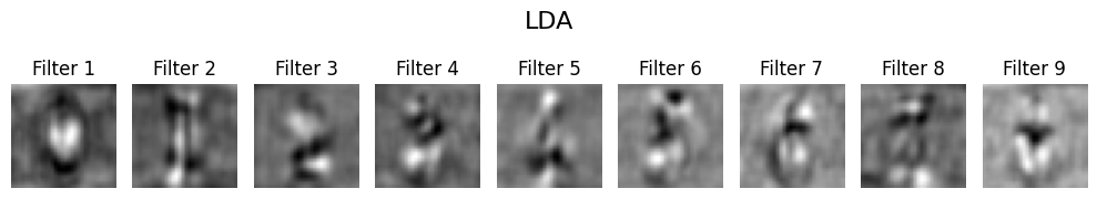
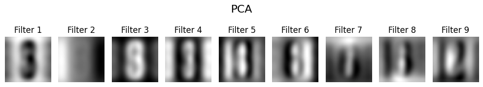
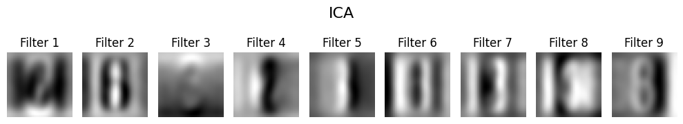
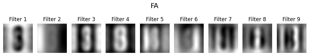
The features learned by the three models look different. First, unsurprisingly, the filters learned by supervised methods LDA and SQFA focus mostly on the digits, while the filters learned by the unsupervised methods have a considerable fraction of their weights in the background. Second, SQFA filters have a more digit-like structure than the rest of the methods.

Filter initialization

A good initialization of the filters can considerably speed up the learning process. The method fit_pca of the SQFA class sets the filters to the PCA components of the data.

Lets evaluate how well the filters separate the classes quadratically, by using a QDA classifier on each feature set. QDA fits a Gaussian distribution (mean and covariance) to each class and uses the Bayes rule to classify samples. Both the class specific means and covariances are used to classify samples.

def get_qda_accuracy(x_train, y_train, x_test, y_test, filters):
    """Fit QDA model to the training data and return the accuracy on the test data."""
    # Get the features
    filters = torch.as_tensor(filters, dtype=torch.float)
    z_train = torch.matmul(x_train, filters.T)
    z_test = torch.matmul(x_test, filters.T)
    # Fit QDA model
    qda = QuadraticDiscriminantAnalysis()
    qda.fit(z_train, y_train)
    y_pred = qda.predict(z_test)
    accuracy = torch.mean(torch.as_tensor(y_pred == y_test.numpy(), dtype=torch.float))
    return accuracy

accuracies = []

for name, filters in zip(model_names, model_filters):
    accuracy = get_qda_accuracy(x_train, y_train, x_test, y_test, filters)
    accuracies.append(accuracy.item() * 100)

# Plot accuracies
fig, ax = plt.subplots(figsize=(6, 3))
plt.bar(range(len(accuracies)), accuracies)
plt.xticks(range(len(accuracies)), model_names, fontsize=12)
plt.yticks(fontsize=12)
plt.ylabel("QDA Accuracy (%)", fontsize=14)
plt.xlabel("Features", fontsize=14)
# Print the accuracies on top of the bars
for i, acc in enumerate(accuracies):
    plt.text(i, acc + 1, f"{acc:.1f}%", ha='center', fontsize=12)
plt.tight_layout()
ax.set_ylim([0, 100])
plt.show()

/home/docs/checkouts/readthedocs.org/user_builds/sqfa/envs/stable/lib/python3.11/site-packages/sklearn/discriminant_analysis.py:1024: LinAlgWarning: The covariance matrix of class 1 is not full rank. Increasing the value of parameter `reg_param` might help reducing the collinearity.
  warnings.warn(
/home/docs/checkouts/readthedocs.org/user_builds/sqfa/envs/stable/lib/python3.11/site-packages/sklearn/discriminant_analysis.py:1024: LinAlgWarning: The covariance matrix of class 2 is not full rank. Increasing the value of parameter `reg_param` might help reducing the collinearity.
  warnings.warn(
/home/docs/checkouts/readthedocs.org/user_builds/sqfa/envs/stable/lib/python3.11/site-packages/sklearn/discriminant_analysis.py:1024: LinAlgWarning: The covariance matrix of class 3 is not full rank. Increasing the value of parameter `reg_param` might help reducing the collinearity.
  warnings.warn(
/home/docs/checkouts/readthedocs.org/user_builds/sqfa/envs/stable/lib/python3.11/site-packages/sklearn/discriminant_analysis.py:1024: LinAlgWarning: The covariance matrix of class 5 is not full rank. Increasing the value of parameter `reg_param` might help reducing the collinearity.
  warnings.warn(

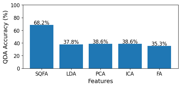
We see that SQFA outperforms all other methods by a large margin in terms of classification accuracy. This is not surprising with respect to the unsupervised methods, since the goal of these methods is not to separate the classes. With respect to LDA, it is also not surprising that taking into account the class-conditional covariances leads to better performance (although the need to estimate a covariance matrix for each class can make SQFA more prone to overfitting in the absence of proper regularization).

SQFA learned the best filters for quadratic discrimination in this task, but is its computational cost reasonable? Let’s compare the time it took to learn the filters for each method.

model_times = [sqfa_time, lda_time, pca_time, ica_time, fa_time]

fig, ax = plt.subplots(figsize=(6, 3))
plt.bar(range(len(model_times)), model_times)
plt.xticks(range(len(model_times)), model_names, fontsize=12)
plt.yticks(fontsize=12)
plt.ylabel("Training Time (s)", fontsize=14)
plt.xlabel("Model", fontsize=14)
# Make y axis logarithmic
plt.yscale('log')
# Print the times on top of the bars
for i, training_time in enumerate(model_times):
    plt.text(i, training_time * 1.5, f"{training_time:.2f}", ha='center', fontsize=12)
plt.tight_layout()
plt.ylim([min(model_times)*0.5, max(model_times) * 5])
plt.show()

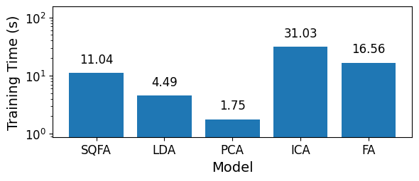
We see that SQFA took approximately the same time as LDA to learn the filters. The relative cost will depend on, but the fact that SQFA is on par with LDA in terms of computational cost indicate that it can be a good tool to use in practice.

In conclusion, SQFA can learn features that allow to discriminate between classes in complex real-world datasets, and it can do so at low computational cost.