Using different distances in SQFA

In the geometry tutorial we explained the geometric intuition behind SQFA and smSQFA. Without much motivation, we proposed using the affine invariant distance in the SPD manifold for smSQFA, and the Fisher-Rao distance in the manifold of normal distributions for SQFA. In the SQFA paper we provide a theoretical and empirical motivation for this choice. However, there are other possible distances (or discriminability measures, or divergences) that could be used instead, either for practical or theoretical reasons.

In this tutorial we show how to use user-defined distances in SQFA and smSQFA with the sqfa package. We will use the opportunity to compare our proposed distances with the Wasserstein distance, which is a popular choice in machine learning[1].

Riemannian metrics vs distances

We use the terms “metric” and “distance” somewhat interchangeably in this tutorial, but they are not the same.

In simplified terms, we can think of the metric as telling us how to measure speeds of curves on the manifold. Like in Euclidean space, the length of a curve is obtained by integrating the speed along the curve. The distance between two points in a Riemannian manifold is the length of the shortest curve connecting them.

The metric is the more fundamental concept in differential geometry, and a given metric defines a distance function on the manifold. Because the metric is more fundamental, we often use the term “metric” to refer to the geometry that we are using, although what we really care about in SQFA is the distance function.

smSQFA: Distances in the SPD manifold

The affine invariant distance between two SPD matrices \(\mathbf{A}\) and \(\mathbf{B}\) is defined as:

\[d_{AI}(\mathbf{A}, \mathbf{B}) = \sqrt{\sum_{k=1}^c \log^2(\lambda_k)} = \| \log(\mathbf{A}^{-1/2} \mathbf{B} \mathbf{A}^{-1/2}) \|_F\]

where in the first definition \(\lambda_k\) is the \(k\)-th generalized eigenvalue of the pair \((\mathbf{A},\mathbf{B})\), and in the second definition \(\|\|_F\) is the Frobenius norm, \(\log\) is the matrix logarithm, and \(\mathbf{A}^{-1/2}\) is the matrix inverse square root of \(\mathbf{A}\).

Affine invariant metric and Fisher-Rao metric for Gaussian distributions

The Fisher-Rao metric is a Riemannian metric in manifolds of probability distributions (i.e. where each point is a probability distribution). Under the Fisher-Rao metric, the squared “speed” of a curve at a given point \(\theta\) (where \(\theta\) is the parameter vector of the distribution) is given by the Fisher information of \(\theta\) along the direction of the curve.

Fisher information is a measure of how discriminable is an infinitesimal change in the parameter \(\theta\) of the distribution. This means that, when using the Fisher-Rao metric, the length of a curve is given by the accumulated discriminability of the infinitesimal changes along the curve.

Interestingly, the affine invariant metric for SPD matrices is equivalent to the Fisher-Rao metric for zero-mean Gaussian distributions. Thus, the affine invariant distance applied to second-moment matrices has some intepretability in terms of probability distributions: it is the accumulated discriminability of the infinitesimal changes transforming \(\mathcal{N}(\mathbf{0}, \mathbf{A})\) into \(\mathcal{N}(\mathbf{0}, \mathbf{B})\).

The Bures-Wasserstein distance between two SPD matrices \(\mathbf{A}\) and \(\mathbf{B}\) is defined as: \(d_{BW}(\mathbf{A}, \mathbf{B}) = \sqrt{ \text{Tr}(\mathbf{A}) + \text{Tr}(\mathbf{B}) - 2 \text{Tr}(\sqrt{\mathbf{A}^{1/2} \mathbf{B} \mathbf{A}^{1/2}}) }\)

where \(\text{Tr}\) is the trace.

Bures-Wasserstein distance and optimal transport

Like the affine invariant distance, the Bures-Wasserstein distance in the SPD manifold has an interpretation in terms of Gaussian distributions. Specifically, the Bures-Wasserstein distance between two SPD matrices \(\mathbf{A}\) and \(\mathbf{B}\) is the optimal transport distance between the two zero-mean Gaussian distributions \(\mathcal{N}(\mathbf{0}, \mathbf{A})\) and \(\mathcal{N}(\mathbf{0}, \mathbf{B})\).

The optimal transport distance is also known as the earth mover’s distance, and it can be thought of as the cost of moving the mass from one distribution to the other. That is, imagine that the Gaussian distribution given by \(\mathcal{N}(\mathbf{0}, \mathbf{A})\) is a pile of dirt. The Bures-Wasserstein distance is the cost of moving that pile of dirt into the shape given by \(\mathcal{N}(\mathbf{0}, \mathbf{B})\). From the earth mover’s perspective we can get some intuition about the Bures-Wasserstein distance. For example, that it is not invariant to scaling: if we scale up the distributions, need to move the dirt across larger distances, increasing the cost.

Optimal transport distances are a popular tool in machine learning, and sometimes have advantages with respect to the Fisher-Rao distances.

Implementing the Bures-Wasserstein distance

The affine invariant distance is already implemented in sqfa.distances.affine_invariant(), so let’s go ahead and implement the Bures-Wasserstein distance in a way that can be used with sqfa.

There are two important requirements for our distance function to be compatible with the smSQFA implementation in sqfa:

1. The distance function should be implemented in PyTorch, because optimization is done with PyTorch.

2. The distance function should take as input two tensors of \(m\)-by-\(m\) matrices with batch dimensions batch_A and batch_B, and return a tensor of pairwise distances with shape (batch_A, batch_B). That is, the two inputs should have shape (batch_A, m, m) and (batch_B, m, m) (where m is variable), and the output should have shape (batch_A, batch_B).

Let’s implement a function to compute the Bures-Wasserstein distance that satisfies these requirements[2] (we implement separate functions for the squared distance and the distance, which will be convenient later):

import torch
import sqfa

torch.manual_seed(9) # Set seed for reproducibility

# IMPLEMENT BURES WASSERSTEIN SQUARED DISTANCE
def bw_distance_sq(A, B):
    """Compute the Bures-Wasserstein distance between all pairs
    of matrices in A and B."""
    tr_A = torch.einsum('ijj->i', A)
    tr_B = torch.einsum('ijj->i', B)

    A_sqrt = sqfa.linalg.spd_sqrt(A) # sqfa provides a stable implementation
    C = sqfa.linalg.conjugate_matrix(B, A_sqrt) # sqfa provides an efficient batch implementation
    C_sqrt_eigvals = torch.sqrt(torch.linalg.eigvalsh(C))
    tr_C = torch.sum(C_sqrt_eigvals, dim=-1)

    bw_distance_sq = tr_A[None,:] + tr_B[:,None] - 2 * tr_C # Use batch broadcasting

    return bw_distance_sq

# IMPLEMENT BURES WASSERSTEIN DISTANCE
def bw_distance(A, B):
    """Compute the Bures-Wasserstein distance between all pairs
    of matrices in A and B."""
    return torch.sqrt(torch.abs(bw_distance_sq(A, B)) + 1e-6) # Add epsilon for gradient stability

Toy problem to compare distances

To test the distances and show how to use them in sqfa, we need some data. We next implement a toy problem to illustrate the difference between the affine invariant distance and the Bures-Wasserstein distance.

Like in the Feature selection tutorial, we will generate a set of covariance matrices for the data of different classes. The problem has 4 dimensional data and 3 classes, all which have zero mean. The 4D data space is designed so that there are two different 2D subspaces, each preferred by one of the two distances when used in smSQFA. The two subspaces are as follows:

1. Dimensions 1 and 2 have different covariance across the classes. The covariances are rotated versions of each other.

2. Dimensions 3 and 4 also have different covariances that are rotated versions of each other. Each covariance also has the same aspect ratio as the covariances in dimensions (1,2). However, the covariances are rotated less than the covariances in dimensions (1,2), but they are also scaled by multiplying them all by the same scalar.

While multiplying all covariances by a scalar in dimensions (3,4) does not change discriminability, having them rotate less makes them less discriminative. So, dimensions (1,2) are more discriminative than dimensions (3,4).

Let’s generate the data and visualize it.

import matplotlib.pyplot as plt

torch.manual_seed(9) # Set seed for reproducibility
n_dim_pairs = 2

# DEFINE THE FUNCTIONS TO GENERATE THE COVARIANCE MATRICES

def make_rotation_matrix(theta, dims):
    """Make a matrix that rotates 2 dimensions of a 6x6 matrix by theta.
    
    Args:
        theta (float): Angle in degrees.
        dims (list): List of 2 dimensions to rotate.
    """
    theta = torch.deg2rad(theta)
    rotation = torch.eye(n_dim_pairs*2)
    rot_mat_2 = torch.tensor([[torch.cos(theta), -torch.sin(theta)],
                              [torch.sin(theta), torch.cos(theta)]])
    for row in range(2):
        for col in range(2):
            rotation[dims[row], dims[col]] = rot_mat_2[row, col]
    return rotation

def make_rotated_classes(base_cov, angles, dims):
    """Rotate 2 dimensions of base_cov, specified in dims, by the angles in the angles list
    Args:
        base_cov (torch.Tensor): Base covariances
        theta (float): Angle in degrees.
        dims (list): List of 2 dimensions to rotate.
    """
    if len(angles) != base_cov.shape[0]:
        raise ValueError('The number of angles must be equal to the number of classes.')

    for i, theta in enumerate(angles):
        rotation_matrix = make_rotation_matrix(theta, dims)
        base_cov[i] = torch.einsum('ij,jk,kl->il', rotation_matrix, base_cov[i], rotation_matrix.T)
    return base_cov

# GENERATE THE COVARIANCE MATRICES

# Define the rotation angles for each class and dimension pair
rotation_angles = [
  [0, 40, 80], # Dimensions 1, 2
  [0, 20, 40],  # Dimensions 3, 4
]

# Generate the baseline covariance to be rotated
n_angles = len(rotation_angles[0])
variances = torch.tensor([0.25, 0.005, 1.0, 0.02])
base_cov = torch.diag(variances) # Initial covariance to be rotated
base_cov = base_cov.repeat(n_angles, 1, 1)

# Generate the rotated covariance matrices for each class
class_covariances = base_cov
for d in range(len(rotation_angles)):
    ang = torch.tensor(rotation_angles[d])
    class_covariances = make_rotated_classes(
      class_covariances, ang, dims=[2*d, 2*d+1]
    )

# VISUALIZE THE COVARIANCE MATRICES

# Function to plot the covariance matrices
def plot_data_covariances(ax, covariances, means=None, lims=None):
    """Plot the covariances as ellipses."""
    if means is None:
        means = torch.zeros(covariances.shape[0], covariances.shape[1])
    n_classes = means.shape[0]

    dim_pairs = [[0, 1], [2, 3]]
    legend_type = ['none', 'discrete']
    for i in range(len(dim_pairs)):
        # Plot ellipses 
        sqfa.plot.statistics_ellipses(ellipses=covariances, centers=means,
                                      dim_pair=dim_pairs[i], ax=ax[i])
        # Plot points for the means
        sqfa.plot.scatter_data(data=means, labels=torch.arange(n_classes),
                               dim_pair=dim_pairs[i], ax=ax[i])
        dim_pairs_label = [d+1 for d in dim_pairs[i]]
        ax[i].set_title(f'Data space (dim {dim_pairs_label})', fontsize=12)
        ax[i].set_aspect('equal')
        if lims is not None:
            ax[i].set_xlim(lims)
            ax[i].set_ylim(lims)

figsize = (8, 4)
lims = (-2.2, 2.2)
fig, ax = plt.subplots(1, n_dim_pairs, figsize=figsize, sharex=True, sharey=True)
plot_data_covariances(ax, class_covariances, lims=lims)
plt.tight_layout()
plt.show()

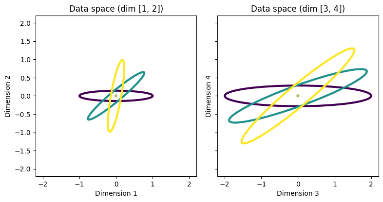
Visually, it should be clear that dimensions (1,2) are more discriminative than dimensions (3,4).

Using the distances in smSQFA

In this section we show how to use the distances in smSQFA. However, before we do that, let’s test that the inputs and outputs of our custom Bures-Wasserstein distance function are as required.

The variable class_covariances that has the covariance matrices for each class has shape (3, 4, 4), where the first dimension is the batch dimensions, and the second and third dimensions are the dimensions of the covariance matrices. Let’s compute the Bures-Wasserstein distance between all pairs of covariance matrices.

# COMPUTE BW DISTANCES
bw_dist = bw_distance(
  A=class_covariances, B=class_covariances
)
print(bw_dist)

tensor([[0.0010, 0.4713, 0.8834],
        [0.4713, 0.0013, 0.4713],
        [0.8834, 0.4714, 0.0016]])

We see that the output has shape (3, 3), which is what we expected since both inputs had shape (3, 4, 4). We also note that the diagonal elements, which have the self-distances, are not zero, partly because we added a small epsilon inside the square root of the distance for gradient stability.

Let’s next learn 2 filters with smSQFA using both the affine invariant distance and the Bures-Wasserstein distance. For this, we use the distance_fun argument of the sqfa.model.SecondMomentsSQFA class, which implements smSQFA.

noise = 0.01 # Regularization noise
n_dim = class_covariances.shape[-1]

# LEARN FILTERS WITH AI DISTANCE
sqfa_ai = sqfa.model.SecondMomentsSQFA(
  n_dim=n_dim,
  n_filters=2,
  feature_noise=noise,
  distance_fun=sqfa.distances.affine_invariant,
)
sqfa_ai.fit(data_statistics=class_covariances, show_progress=False)
ai_filters = sqfa_ai.filters.detach()

# LEARN FILTERS WITH BW DISTANCE
sqfa_bw = sqfa.model.SecondMomentsSQFA(
  n_dim=n_dim,
  n_filters=2,
  feature_noise=noise,
  distance_fun=bw_distance,
)
sqfa_bw.fit(data_statistics=class_covariances, show_progress=False)
bw_filters = sqfa_bw.filters.detach()

Loss change below 1e-06 for 3 consecutive epochs. Stopping training at epoch 10/300.

Loss change below 1e-06 for 3 consecutive epochs. Stopping training at epoch 14/300.

Let’s visualize the filters as arrows pointing in the data space:

import matplotlib.patches as mpatches
# Function to plot filters on top of the data covariances
def plot_filters(ax, filters, color, name):
    """Plot the filters as arrows in data space."""
    awidth = 0.05
    n_filters = 2
    n_subspaces = 2
    for f in range(n_filters):
        for s in range(n_subspaces):
            if torch.norm(filters[f, s*2:(s*2+2)]) > 1e-2: # Omit if filter is ~zero
                label = name if f==0 else None
                ax[s].arrow(
                    0, 0,
                    filters[f, s*2], filters[f, s*2+1],
                    width=awidth,
                    head_width=awidth*5,
                    label=label,
                    color=color
                )

# Initialize plot and plot statistics
figsize = (8, 3)
fig, ax = plt.subplots(1, 2, figsize=figsize, sharex=True, sharey=True)
plot_data_covariances(ax, class_covariances, lims=lims)

# PLOT THE FILTERS
plot_filters(ax, ai_filters, 'k', 'AI')
plot_filters(ax, bw_filters, 'r', 'BW')

# Add legend
ai_patch = mpatches.Patch(color='k', label='AI')
bw_patch = mpatches.Patch(color='r', label='BW')
fig.legend(handles=[ai_patch, bw_patch], loc='center right')
plt.show()

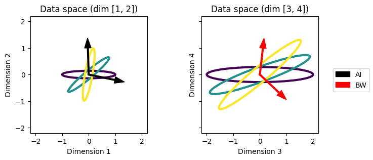
We see that the filters learned with the affine invariant distance are aligned with the most discriminative dimensions (1,2), while the filters learned with the Bures-Wasserstein distance are aligned with the less discriminative dimensions (3,4).

Why do Bures-Wasserstein filters select for the less discriminative dimensions? Using the earth mover’s intuition of the Bures-Wasserstein distance, we can see that the BW distance is not scale-invariant. In our toy problem, the scaling used in the dimensions (3,4) makes the cost of moving the dirt from one distribution to the other higher, even though it does not change discriminability. This gives us an intuition of why the Bures-Wasserstein distance might not prioritize the most discriminable features.

This is a good example of how the choice of distance function is crucial in the success of the feature learning process.

SQFA: Distances between first- and second-moment statistics

In the previous sections we discussed distances in smSQFA, which uses only second-moment matrices. Now we move to SQFA, which considers distances between the classes using both first- and second-moment statistics.

To take distances between classes using first- and second-moment statistics, we can use the manifold of Gaussian distributions, which we denote as \(\mathcal{M}_{\mathcal{N}}\). In this manifold, each point corresponds to a normal distribution \(\mathcal{N}(\mu, \Sigma)\), and it is parametrized by the mean \(\mu\) and the covariance \(\Sigma\).

In the SQFA paper, we propose using as the distance between classes \(i\) and \(j\) the Fisher-Rao distance between \(\mathcal{N}(\mu_i, \Sigma_i)\) and \(\mathcal{N}(\mu_j, \Sigma_j)\) in \(\mathcal{M}_{\mathcal{N}}\). Unfortunately, this distance does not have a closed-form expression, so we used a lower-bound approximation developed by Calvo and Oller (1990)[3]. This approximation is implemented in sqfa.distances.fisher_rao_lower_bound().

Implementing the Wasserstein distance in \(\mathcal{M}_{\mathcal{N}}\)

Let’s implement the Wasserstein L2 distance in \(\mathcal{M}_{\mathcal{N}}\). This distance is given by \(d_{W}(\mathcal{N}(\mu_i, \Sigma_i), \mathcal{N}(\mu_j, \Sigma_j)) = \sqrt{ \| \mu_i - \mu_j \|^2 + \text{Tr}(\mathbf{\Sigma_i}) + \text{Tr}(\mathbf{\Sigma_j}) - 2 \text{tr}(\sqrt{\mathbf{\Sigma_i}^{1/2} \mathbf{\Sigma_j} \mathbf{\Sigma_i}^{1/2}}) }\)

Note that the second term inside the square root is the Bures-Wasserstein squared distance between the covariance matrices \(\Sigma_i\) and \(\Sigma_j\).

Like for smSQFA, there are requirements for a custom distance function to be compatible with SQFA:

1. The distance function should be implemented in PyTorch.

2. The distance function should take as input two dictionaries with keys means and covariances. Each key should have a tensor as value. The tensor for means should have shape (batch_A, n_dim) and the tensor for covariances should have shape (batch_A, n_dim, n_dim) (or batch_B) for the second input). The function should return a tensor of pairwise distances with shape (batch_A, batch_B).

We implement the new distance making use of our implementation of the Bures-Wasserstein distance:

# IMPLEMENT WASSERSTEIN DISTANCE IN M_N
def wasserstein_distance(statistics_A, statistics_B):
    """Compute the Wasserstein distance between all pairs
    of distributions in (mu, Sigma) and (mu2, Sigma2)."""

    mean_A = statistics_A['means']
    mean_B = statistics_B['means']
    dist_means_sq = torch.sum((mean_A[:, None] - mean_B[None, :]) ** 2, dim=-1)

    dist_covariances_sq = bw_distance_sq(
        A=statistics_A['covariances'], B=statistics_B['covariances']
    )
    
    distance = torch.sqrt(torch.abs(dist_means_sq + dist_covariances_sq) + 1e-6) 

    return distance

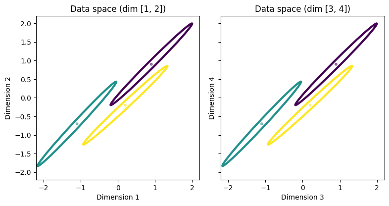
Toy problem to compare distances in \(\mathcal{M}_{\mathcal{N}}\)

To compare the distances in \(\mathcal{M}_{\mathcal{N}}\) we will generate a toy problem similar to the one used in the previous section. The problem will have 4 dimensional data and 3 classes. Again, there will be two 2D subspaces, but unlike the previous example, these two subspaces are identical, and the difference between the distances will be seen within the subspaces.

In each 2D subspace, the covariance ellipses have an enlongated shape, with a high-variance direction and a low-variance direction. In each subspace, the means of the classes are different. The differences between the means are smaller in the direction of low-variance, and larger in the direction of high-variance. However, the larger differences in the means are not enough to compensate for the much larger variance in the high-variance direction.

The intuition is that the Fisher-Rao distance will prefer the directions with smaller variance, which despite having smaller differences in the means, are more discriminative. The earth mover’s intuition again tells us that the Wasserstein distance will prefer the high-variance directions, which are less discriminative.

Let’s generate the data and visualize it.

# GENERATE THE COVARIANCE MATRICES
rotation_angles = [
  [45, 47, 43], # Dimensions 1, 2
  [45, 47, 43],  # Dimensions 3, 4
]

# Generate the baseline covariance to be rotated
n_angles = len(rotation_angles[0])
variances = torch.tensor([0.6, 0.002, 0.6, 0.002])
base_cov = torch.diag(variances) # Initial covariance to be rotated
base_cov = base_cov.repeat(n_angles, 1, 1)

# Generate the rotated covariance matrices for each class
class_covariances = base_cov
for d in range(len(rotation_angles)):
    ang = torch.tensor(rotation_angles[d])
    class_covariances = make_rotated_classes(
      class_covariances, ang, dims=[2*d, 2*d+1]
    )

# GENERATE THE MEAN VECTORS
small = 0.2
large = 0.9
class_means = torch.as_tensor([
    [large, large, large, large],
    [-small - large, small - large, -small - large, small - large],
    [small, -small, small, -small],
])

# VISUALIZE THE COVARIANCE MATRICES
figsize = (8, 4)
lims = (-2.2, 2.2)
fig, ax = plt.subplots(1, n_dim_pairs, figsize=figsize, sharex=True, sharey=True)
plot_data_covariances(ax, class_covariances, means=class_means, lims=lims)
plt.tight_layout()
plt.show()

Let’s test that the inputs and outputs of our custom Wasserstein distance function are as required.

# COMPUTE WASSERSTEIN DISTANCES
data_statistics = {
  "means": class_means,
  "covariances": class_covariances,
}

wasserstein_dist = wasserstein_distance(
  statistics_A=data_statistics, statistics_B=data_statistics
)

print(wasserstein_dist)

tensor([[3.0957e-03, 3.6224e+00, 1.8443e+00],
        [3.6224e+00, 2.7705e-03, 1.9712e+00],
        [1.8443e+00, 1.9712e+00, 2.7705e-03]])

We see that the output has shape (3, 3), which is what we expected. Now, let’s learn 2 filters with SQFA using both the Fisher-Rao (lower-bound) distance and the Wasserstein distance. For this, we again use the parameter distance_fun when creating the sqfa.model.SQFA object.

# LEARN FILTERS WITH FISHER-RAO DISTANCE
noise = 0.001
sqfa_fr = sqfa.model.SQFA(
  n_dim=n_dim,
  n_filters=2,
  feature_noise=noise,
  distance_fun=sqfa.distances.fisher_rao_lower_bound,
)
sqfa_fr.fit(data_statistics=data_statistics, show_progress=False)
fr_filters = sqfa_fr.filters.detach()

# LEARN FILTERS WITH WASSERSTEIN DISTANCE
sqfa_w = sqfa.model.SQFA(
  n_dim=n_dim,
  n_filters=2,
  feature_noise=noise,
  distance_fun=wasserstein_distance,
)
sqfa_w.fit(data_statistics=data_statistics, show_progress=False)
w_filters = sqfa_w.filters.detach()

Loss change below 1e-06 for 3 consecutive epochs. Stopping training at epoch 15/300.

Loss change below 1e-06 for 3 consecutive epochs. Stopping training at epoch 10/300.

Let’s visualize the filters as arrows pointing in the data space:

# Initialize plot and plot statistics
figsize = (8, 3)
fig, ax = plt.subplots(1, 2, figsize=figsize, sharex=True, sharey=True)
plot_data_covariances(ax, class_covariances, class_means, lims=lims)

# PLOT THE FILTERS
plot_filters(ax, fr_filters, 'k', 'FR')
plot_filters(ax, w_filters, 'r',  'Wass')

# Add legend
fr_patch = mpatches.Patch(color='k', label='FR')
w_patch = mpatches.Patch(color='r', label='Wass')
fig.legend(handles=[fr_patch, w_patch], loc='center right')
plt.show()

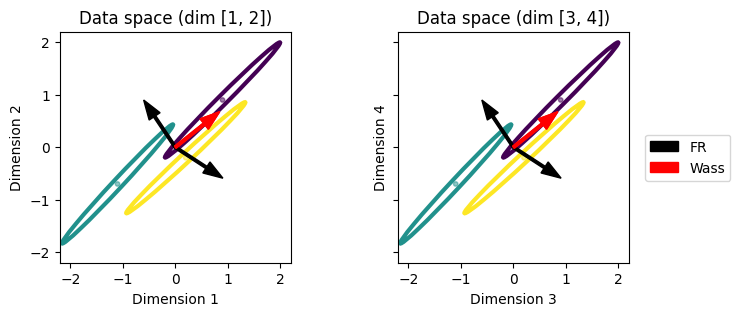
It might seem that there are 4 filters in the plot, but that is not the case. Note that each filter is a 4-dimensional vector, so a single filter might can require an arrow in each 2D subspace to be visualized.

We see that, in each 2D subspace, the filters learned with the Fisher-Rao distance point in the direction of highest discriminability, while the filters learned with the Wasserstein distance point in the direction of highest variance. Thus, again the Fisher-Rao distance is more successful in selecting the most discriminative features.

Let’s plot the output of the filters like we did in the Feature selection tutorial:

# GET THE FEATURE STATISTICS

fr_covariances = sqfa_fr.transform_scatters(
  data_statistics["covariances"]
).detach()
fr_means = sqfa_fr.transform(
  data_statistics["means"]
).detach()

w_covariances = sqfa_w.transform_scatters(
  data_statistics["covariances"]
).detach()
w_means = sqfa_w.transform(
  data_statistics["means"]
).detach()

feature_covs = [fr_covariances, w_covariances]
feature_means = [fr_means, w_means]
model_names = ['Fisher-Rao', 'Wasserstein']

# PLOT FEATURE STATISTICS
for i in range(len(model_names)):
    fig, ax = plt.subplots(1, 1, figsize=(2.5, 2.5))
    covs = feature_covs[i]
    means = feature_means[i]
    sqfa.plot.statistics_ellipses(ellipses=covs, centers=means, ax=ax)
    ax.set_title(f'{model_names[i]} feature-space')
    ax.set_xlabel(f'{model_names[i]} feature 1')
    ax.set_ylabel(f'{model_names[i]} feature 2')
    plt.show()

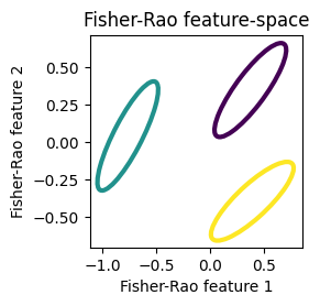
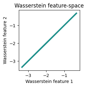
We see that the classes are well separated in the feature space of the Fisher-Rao filters, while the classes are not well separated in the feature space of the Wasserstein filters. What’s more, although not visible in the plot with arrows, it turns out that both Wasserstein filters are parallel to each other. Let’s print the values of the filters to see this:

print('Fisher-Rao filters:')
print(fr_filters)
print('Wasserstein filters:')
print(w_filters)

Fisher-Rao filters:
tensor([[ 0.5928, -0.3854,  0.5928, -0.3854],
        [-0.3935,  0.5875, -0.3935,  0.5875]])
Wasserstein filters:
tensor([[0.5522, 0.4417, 0.5522, 0.4417],
        [0.5522, 0.4417, 0.5522, 0.4417]])

Thus, the Wasserstein distance is not only less discriminative than the Fisher-Rao distance, but it also learns degenerate filters in this example.

Conclusion

In this tutorial we have shown how to use custom distances in SQFA. We have also seen that the choice of distance function is crucial in the success of the feature learning process. In particular, we showed that the Fisher-Rao distance is more successful at learning discriminative features than the Wasserstein distance, which is also a popular choice in machine learning.

---

[1]

More distances are tested in the SQFA paper. Link: https://arxiv.org/abs/2502.00168

[2]

For efficiency in implementing the squared distance we use a couple of linear algebra tricks. First, we use that \(\text{tr}(M)\) is the sum of the eigenvalues of \(M\). Then, we use that \(A^{1/2} B A^{1/2}\) is SPD, because \(A^{1/2}\) is symmetric, and any SPD matrix \(M\) and invertible matrix \(G\) satisfy that \(G M G^T\) is SPD. Finally, we use that for an SPD matrix \(M\), the eigenvalues of \(\sqrt{M}\) are the square roots of the eigenvalues of \(M\). Thus, we have that \(\text{tr}(A^{1/2} B A^{1/2}) = \sum_i \lambda_i^{1/2}\), where \(\lambda_i\) are the eigenvalues of \(A^{1/2} B A^{1/2}\).

[3]

Calvo, B., & Oller, J. (1990). “A distance between multivariate normal distributions based in an embedding into the siegel group.” In Journal of Multivariate Analysis (Vol 35, Issue 2, pp 223-242).