Feature selection: SQFA vs PCA vs LDA

In this tutorial we consider a toy problem to compare SQFA to other standard feature learning techniques, Principal Component Analysis (PCA), and Linear Discriminant Analysis (LDA).

Description of the toy problem

To illustrate the differences between these methods, we consider a toy problem with 6 dimensional data and 3 classes. This toy problem is designed so that in the 6D data space there are three different 2D subspaces, each of which is preferred by one of the three methods. These three subspaces are as follows:

1. Dimensions 1 and 2 have zero mean for all classes, but different covariance matrices that allow for good quadratic separability of the classes. The covariances of the classes are rotated versions of each other. The differences in covariances make this space preferred by SQFA and smSQFA. But because the means are the same, this subspace is not preferred by LDA. The overall variance in this subspace is moderate, so PCA does not prefer it either.

2. Dimensions 3 and 4 have slightly different means for the classes, but the same covariance matrix. The differences in means make this space preferred by LDA. The overall variance in this subspace is moderate, so PCA does not prefer it. The differences in the class means are small, so this subspace is not very discriminative.

3. Dimensions 5 and 6 have the same mean and covariance matrix for all classes, but high overall variance. This space is preferred by PCA. This subspace is not preferred by SQFA or LDA because it is not discriminative.

The three subspaces will be made clear in the plots below.

Implementation of the toy problem

We next implement the means and covariances of the classes described above.

import torch
import sqfa
import matplotlib.pyplot as plt
import matplotlib.patches as mpatches

torch.manual_seed(9) # Set seed for reproducibility

# GENERATE 6D COVARIANCES
# Define the functions to generate the rotated covariances
def make_rotation_matrix(theta):
    """Make a matrix that rotates the first 2 dimensions of a 6D tensor"""
    theta = torch.deg2rad(theta)
    rotation = torch.eye(6)
    rotation[:2, :2] = torch.tensor([[torch.cos(theta), -torch.sin(theta)],
                                     [torch.sin(theta), torch.cos(theta)]])
    return rotation

def make_rotated_covariances(base_cov, angles):
    """Take a baseline covariance matrix, and return a set of
    covariances with the first two dimensions rotated by the
    angles in the angles list"""
    covs = torch.as_tensor([])
    for theta in angles:
        rotation_matrix = make_rotation_matrix(theta)
        rotated_cov = torch.einsum('ij,jk,kl->il', rotation_matrix, base_cov, rotation_matrix.T)
        covs = torch.cat([covs, rotated_cov.unsqueeze(0)], dim=0)
    return covs

# Generate the covariance matrices
variances = torch.tensor([0.7, 0.01, 0.5, 0.5, 1.0, 1.0])
base_cov = torch.diag(variances)

angles = torch.as_tensor([15, 45, 70])
class_covariances = make_rotated_covariances(base_cov, angles)

# GENERATE 6D MEANS
class_means = torch.tensor(
  [[0, 0, 0.2, -0.1, 0, 0],
   [0, 0, 0, 0.2, 0, 0],
   [0, 0, -0.2, -0.1, 0, 0]]
)

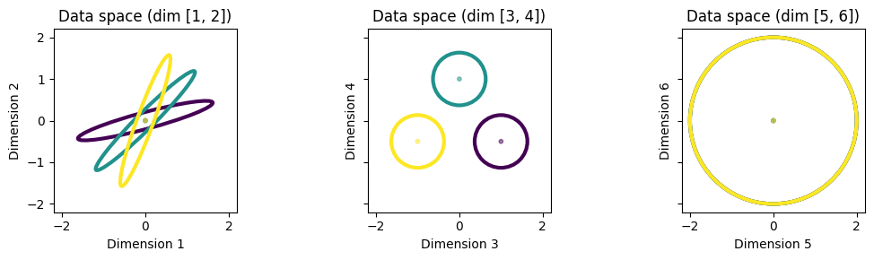
Let’s visualize the class distributions in the 6D data space.

# VISUALIZE THE 3 SUBSPACES
def plot_data_covariances(ax, covariances, means=None):
    """Plot the covariances as ellipses."""
    if means is None:
        means = torch.zeros(covariances.shape[0], covariances.shape[1])

    dim_pairs = [[0, 1], [2, 3], [4, 5]]
    for i in range(len(dim_pairs)):
        # Plot ellipses 
        sqfa.plot.statistics_ellipses(ellipses=covariances, centers=means,
                                      dim_pair=dim_pairs[i], ax=ax[i])
        # Plot points for the means
        sqfa.plot.scatter_data(data=means, labels=torch.arange(3),
                               dim_pair=dim_pairs[i], ax=ax[i])
        dim_pairs_label = [d+1 for d in dim_pairs[i]]
        #ax[i].set_title(f'Data space \n dim {dim_pairs_label}', fontsize=12)
        ax[i].set_title(f'Data space (dim {dim_pairs_label})', fontsize=12)
        ax[i].set_aspect('equal')

figsize = (8, 3)
fig, ax = plt.subplots(1, 3, figsize=figsize, sharex=True, sharey=True)
plot_data_covariances(ax, class_covariances, class_means)
plt.tight_layout()
plt.show()

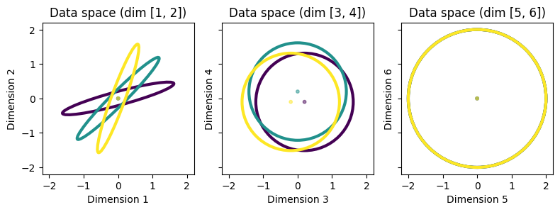
It should be clear from the plot above how the three subspaces should be preferred by the three methods. It should also be clear that the first subspace (dimensions 1 and 2) is the most discriminative.

Learning filters with SQFA, LDA, and PCA

Let’s now learn two filters on this 6D dataset using SQFA, smSQFA, LDA, and PCA, to see whether the filters learned by these methods match our expectations.

We first learn the filters using SQFA and smSQFA. Note how we use as input a dictionary with the means and covariances of the classes.

# Learn SQFA filters
stats_dict = {'means': class_means, 'covariances': class_covariances}
sqfa_model = sqfa.model.SQFA(n_dim=6, n_filters=2, feature_noise=0.01)
sqfa_model.fit(data_statistics=stats_dict, show_progress=False)
sqfa_filters = sqfa_model.filters.detach()

# Learn smSQFA filters
smsqfa_model = sqfa.model.SecondMomentsSQFA(n_dim=6, n_filters=2, feature_noise=0.01)
smsqfa_model.fit(data_statistics=stats_dict, show_progress=False)
smsqfa_filters = smsqfa_model.filters.detach()

Loss change below 1e-06 for 3 consecutive epochs. Stopping training at epoch 17/300.

Loss change below 1e-06 for 3 consecutive epochs. Stopping training at epoch 46/300.

Next, we learn the filters using LDA. We use a custom function for learning LDA filters, since standard implementations of LDA usually take the data as input, rather than the class statistics.

def lda(scatter_between, scatter_within):
    """Compute LDA filters from between class and within class scatter matrices."""
    eigvec, eigval = sqfa.linalg.generalized_eigenvectors(
      scatter_between,
      scatter_within
    )
    eigvec = eigvec[:, eigval>1e-5]
    return eigvec.transpose(-1, -2)

# Get scatter matrices for LDA
scatter_within = torch.mean(class_covariances, dim=0)
scatter_between = class_means.T @ class_means

# Learn LDA
lda_filters = lda(scatter_between, scatter_within)

Finally, we learn the filters using PCA. Again, we use custom code to learn the PCA filters from the dataset statistics. Note that PCA operates on the global scatter matrix of the dataset (i.e. without class-specific statistics), which can be computed by adding the within-class and between-class scatter matrices used for LDA.

# Learn PCA filters
global_scatter = scatter_within + scatter_between
eigval, eigvec = torch.linalg.eigh(global_scatter)
pca_filters = eigvec[:, -2:].T

Visualizing the filters

To visualize the filters learned by the different methods, we plot each filter as an arrow in the original data space, to see how they relate to the data statistics. (We slightly scale the SQFA and smSQFA filters for better visualization, because they perfectly overlap one another.)

# Function to plot filters on top of the data covariances
def plot_filters(ax, filters, color, name):
    """Plot the filters as arrows in data space."""
    awidth = 0.05
    n_filters = 2
    n_subspaces = 3
    for f in range(n_filters):
        for s in range(n_subspaces):
            if torch.norm(filters[f, s*2:(s*2+2)]) > 1e-2: # Omit if filter is ~zero
                label = name if f==0 else None
                ax[s].arrow(
                    0, 0,
                    filters[f, s*2], filters[f, s*2+1],
                    width=awidth,
                    head_width=awidth*5,
                    label=label,
                    color=color
                )

# Initialize plot and plot statistics
figsize = (11, 3)
fig, ax = plt.subplots(1, 3, figsize=figsize, sharex=True, sharey=True)
plot_data_covariances(ax, class_covariances, class_means)

# PLOT THE FILTERS
plot_filters(ax, sqfa_filters*1.1, 'k', 'SQFA')
plot_filters(ax, smsqfa_filters*0.8, 'r', 'smSQFA')
plot_filters(ax, lda_filters, 'b', 'LDA')
plot_filters(ax, pca_filters, 'g', 'PCA')

# Add legend
sqfa_patch = mpatches.Patch(color='k', label='SQFA')
smsqfa_patch = mpatches.Patch(color='r', label='smSQFA')
lda_patch  = mpatches.Patch(color='b', label='LDA')
pca_patch  = mpatches.Patch(color='g', label='PCA')
fig.legend(handles=[sqfa_patch, smsqfa_patch, lda_patch, pca_patch],
           loc='center right')
plt.show()

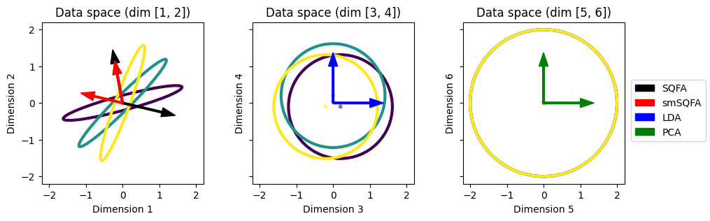
As expected, the SQFA and smSQFA filters (black and red) prefer the subspace with differences in covariances (dimensions 1 and 2). The LDA filters (blue) prefer the subspace with differences in means (dimensions 3 and 4). The PCA filters (green) prefer the subspace with high overall variance (dimensions 5 and 6).

Visualizing the feature statistics

Let’s now visualize the class statistics in the feature space learned by each method. The statistics in the feature space are obtained by projecting the class means and covariances into the filters.

# GET FEATURE COVARIANCES
# There is an in-build method in the sqfa models
sqfa_covariances = sqfa_model.transform_scatters(class_covariances).detach()
smsqfa_covariances = smsqfa_model.transform_scatters(class_covariances).detach()
lda_covariances = torch.einsum('ij,njk,kl->nil', lda_filters, class_covariances, lda_filters.T)
pca_covariances = torch.einsum('ij,njk,kl->nil', pca_filters, class_covariances, pca_filters.T)

# GET FEATURE MEANS
sqfa_means = sqfa_model.transform(class_means).detach()
smsqfa_means = smsqfa_model.transform(class_means).detach()
lda_means = class_means @ lda_filters.T
pca_means = class_means @ pca_filters.T

feature_covs = [sqfa_covariances, smsqfa_covariances, lda_covariances, pca_covariances]
feature_means = [sqfa_means, smsqfa_means, lda_means, pca_means]
model_names = ['SQFA', 'smSQFA', 'LDA', 'PCA']

# PLOT FEATURE STATISTICS
for i in range(len(model_names)):
    fig, ax = plt.subplots(1, 1, figsize=(2.5, 2.5))
    covs = feature_covs[i]
    means = feature_means[i]
    sqfa.plot.statistics_ellipses(ellipses=covs, centers=means, ax=ax)
    ax.set_title(f'{model_names[i]} feature-space')
    ax.set_xlabel(f'{model_names[i]} feature 1')
    ax.set_ylabel(f'{model_names[i]} feature 2')
    plt.show()

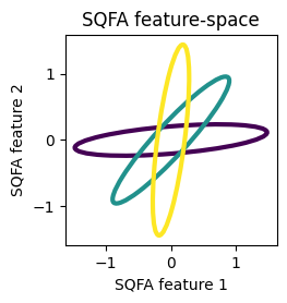
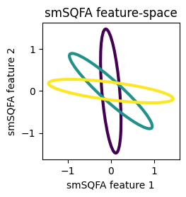
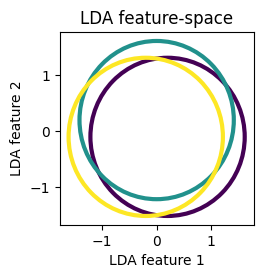
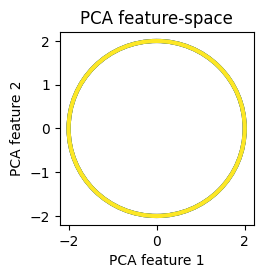
We see that the classes are well separated by their second-order structure in the feature spaces learned by SQFA and smSQFA.

SQFA also accounts for differences in means

In the previous example, the most discriminative subspace was the one with differences in covariances, and this is the subspace that were selected for by SQFA. However, SQFA features can also prefer subspaces with differences in means, when these are more discriminative.

To show how SQFA can flexibly prioritize differences in means or covariances (or combinations of both) to maximize discriminability, we test SQFA on a modified version of the toy problem above. In this modified toy problem, we increase the differences in the means and decrease the variance in the second subspace (dimensions 3 and 4), making this subspace more discriminative than the first one.

# MODIFY THE MEANS AND COVARIANCES
class_means = class_means * 5
class_covariances[:, 2:4, 2:4] = class_covariances[:, 2:4, 2:4] * 0.2

# VISUALIZE THE 3 SUBSPACES
fig, ax = plt.subplots(1, 3, figsize=figsize, sharex=True, sharey=True)
plot_data_covariances(ax, class_covariances, class_means)
plt.tight_layout()
plt.show()

We see that the second subspace (dimensions 3 and 4) is now more discriminative than the first one (dimensions 1 and 2). Let’s now learn the filters using SQFA and smSQFA and visualize them.

# Fill new stats dictionary
stats_dict = {'means': class_means, 'covariances': class_covariances}

# Learn SQFA filters
sqfa_model = sqfa.model.SQFA(n_dim=6, n_filters=2, feature_noise=0.01)
sqfa_model.fit(data_statistics=stats_dict, show_progress=False)
sqfa_filters = sqfa_model.filters.detach()

# Learn smSQFA filters
smsqfa_model = sqfa.model.SecondMomentsSQFA(n_dim=6, n_filters=2, feature_noise=0.01)
smsqfa_model.fit(data_statistics=stats_dict, show_progress=False)
smsqfa_filters = smsqfa_model.filters.detach()

Loss change below 1e-06 for 3 consecutive epochs. Stopping training at epoch 9/300.

Loss change below 1e-06 for 3 consecutive epochs. Stopping training at epoch 16/300.

# PLOT THE FILTERS
fig, ax = plt.subplots(1, 3, figsize=figsize, sharex=True, sharey=True)
plot_data_covariances(ax, class_covariances, class_means)
# PLOT THE FILTERS

plot_filters(ax, sqfa_filters, 'k', 'SQFA')
plot_filters(ax, smsqfa_filters, 'r', 'smSQFA')

# Add legend
sqfa_patch = mpatches.Patch(color='k', label='SQFA')
smsqfa_patch = mpatches.Patch(color='r', label='smSQFA')
fig.legend(handles=[sqfa_patch, smsqfa_patch],
           loc='center right')
plt.show()

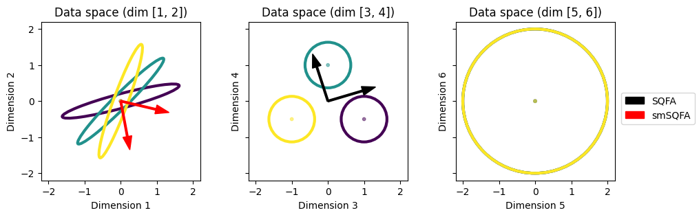
We see that, as expected, SQFA filters now select for the subspace of dimensions 3 and 4, which are more discriminative because of the differences in means. On the other hand, smSQFA, which only maximizes the differences in second-moment matrices again selects for the subspace of dimensions 1 and 2. While second-moment matrices contain information about both means and covariances, it is more informative to consider means and covariances separately, as this example shows.

Conclusion

SQFA learns features that maximize the differences between classes, taking into account both first- and second-order class-conditional statistics. SQFA filters can select for the most discriminative data subspaces whether these are characterized by differences in means, differences in second-order statistics, or both. This is unlike considering only first-order statistics (LDA) or second-moment matrices (smSQFA).